nz_elev = terra::rast(system.file(
  "raster/nz_elev.tif",
  package = "spDataLarge"
))The third of three posts revisiting old data visualization work on TidyTuesday data sets. The code and plot were initially created on November 2nd, 2021. This was an interesting and unusual TidyTuesday, exploring a book instead of a dataset. This week’s exercise was an introduction to geocomputation through the resource, Geocomputation with R. See the TidyTuesday repo for more information.
1 Setup
1.1 (Install) and Load Packages
1.2 Read in data
2 Create some maps
2.1 Add a fill layer to the shape of New Zealand
tm_shape(nz) +
  tm_fill()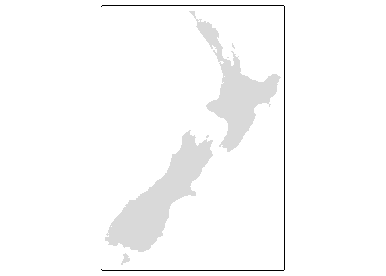
2.2 Draw the borders
tm_shape(nz) +
  tm_borders()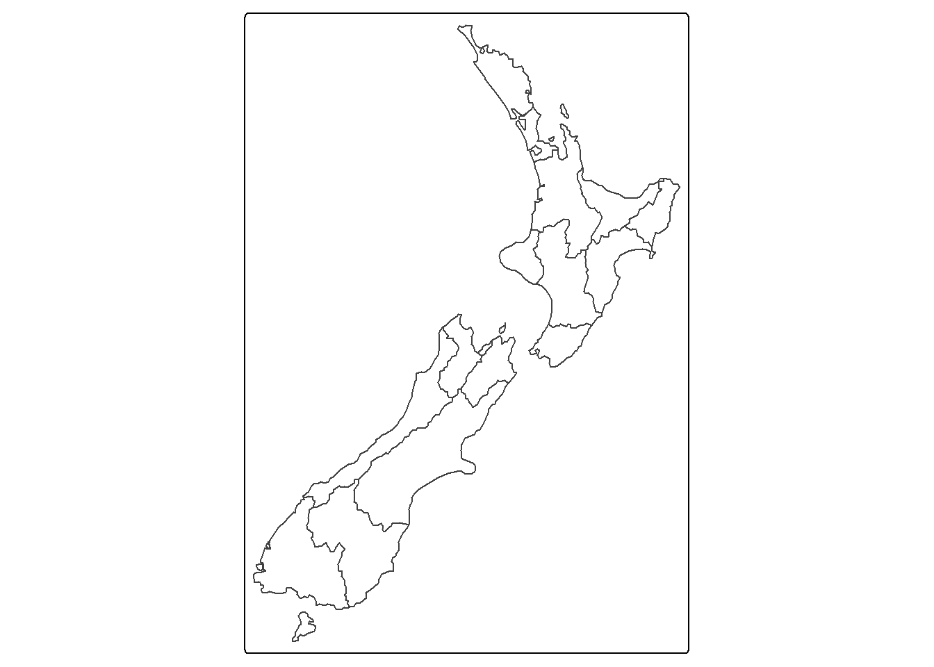
2.3 Combine the fill and borders layers
tm_shape(nz) +
  tm_fill() +
  tm_borders()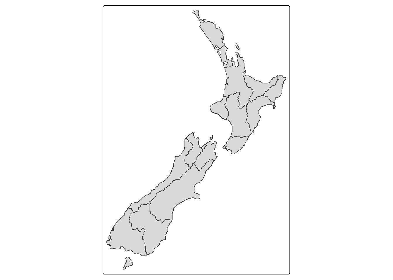
2.4 Display multiple data sources on a map
- Begin with a
map_nz = tm_shape(nz) + tm_polygons()
map_nz
- Add elevation data
map_nz1 = map_nz +
  tm_shape(nz_elev) +
tm_raster(col_alpha = 0.7)- Surround the geometry with a buffer region representing water
nz_water = st_union(nz) %>% st_buffer(22200) %>% st_cast(to = "LINESTRING")

map_nz2 = map_nz1 +
  tm_shape(nz_water) +
tm_lines()- Draw dots at the 101 highest points in New Zealand
map_nz3 = map_nz2 +
  tm_shape(nz_height) +
tm_dots()tmap_arrange(map_nz1, map_nz2, map_nz3)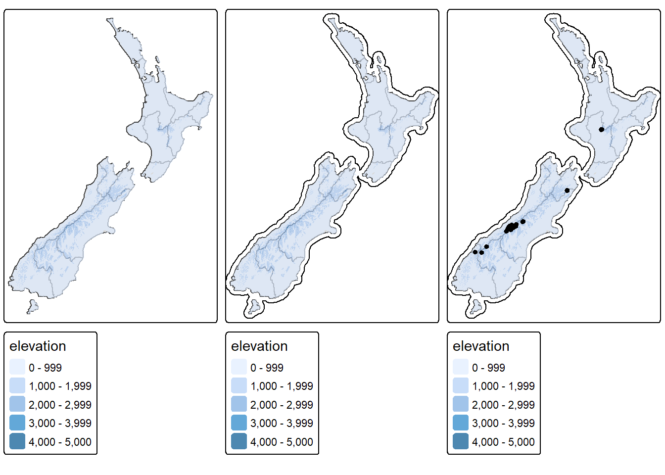
Citation
BibTeX citation:
@online{kasowitz2025,
  author = {Kasowitz, Seth},
  title = {Quick {Plot:} {TidyTuesday} 2021 {Week} 45},
  date = {2025-09-30},
  url = {https://sethkasowitz.com/posts/2025-09-30_revisiting-tidytuesday-2021wk45/},
  langid = {en}
}
For attribution, please cite this work as:
Kasowitz, Seth. 2025. “Quick Plot: TidyTuesday 2021 Week
45.” September 30, 2025. https://sethkasowitz.com/posts/2025-09-30_revisiting-tidytuesday-2021wk45/.