Quick Plot: TidyTuesday 2021 Week 42

The second of three posts revisiting old data visualization work on TidyTuesday data sets. The code and plot were initially created on October 22nd, 2021. The pumpkin weight data was originally sourced from BigPumpkins.com. See the TidyTuesday repo for more information.

1 Setup

1.1 Packages

library(tidyverse)
library(ggridges)
library(ggthemes)
library(tidytext)
library(geofacet)
theme_set(theme_tufte())

1.2 Load Data

tuesdata <- tidytuesdayR::tt_load(2021, week = 43)
pumpkins <- tuesdata$pumpkins

2 Data Prep

glimpse(pumpkins)

Rows: 28,065
Columns: 14
$ id                <chr> "2013-F", "2013-F", "2013-F", "2013-F", "2013-F", "2…
$ place             <chr> "1", "2", "3", "4", "5", "5", "7", "8", "9", "10", "…
$ weight_lbs        <chr> "154.50", "146.50", "145.00", "140.80", "139.00", "1…
$ grower_name       <chr> "Ellenbecker, Todd & Sequoia", "Razo, Steve", "Ellen…
$ city              <chr> "Gleason", "New Middletown", "Glenson", "Combined Lo…
$ state_prov        <chr> "Wisconsin", "Ohio", "Wisconsin", "Wisconsin", "Wisc…
$ country           <chr> "United States", "United States", "United States", "…
$ gpc_site          <chr> "Nekoosa Giant Pumpkin Fest", "Ohio Valley Giant Pum…
$ seed_mother       <chr> "209 Werner", "150.5 Snyder", "209 Werner", "109 Mar…
$ pollinator_father <chr> "Self", NA, "103 Mackinnon", "209 Werner '12", "open…
$ ott               <chr> "184.0", "194.0", "177.0", "194.0", "0.0", "190.0", …
$ est_weight        <chr> "129.00", "151.00", "115.00", "151.00", "0.00", "141…
$ pct_chart         <chr> "20.0", "-3.0", "26.0", "-7.0", "0.0", "-1.0", "-4.0…
$ variety           <chr> NA, NA, NA, NA, NA, NA, NA, NA, NA, NA, NA, NA, NA, …

Some light cleanup will make this pumpkin data easier to visualize.

• Several variables contain numeric data but are character types
• Some missing data (NA) can be dropped
• The id contains two pieces of data that it would be convenient to separate
• There are some rows with wonky data that we should filter out entirely. e.g.

id	place	weight_lbs	grower_name	city	state_prov	country	gpc_site	seed_mother	pollinator_father	ott	est_weight	pct_chart	variety
2021-W	253 Entries. (18 exhibition only, 5 damaged)	253 Entries. (18 exhibition only, 5 damaged)	253 Entries. (18 exhibition only, 5 damaged)	253 Entries. (18 exhibition only, 5 damaged)	253 Entries. (18 exhibition only, 5 damaged)	253 Entries. (18 exhibition only, 5 damaged)	253 Entries. (18 exhibition only, 5 damaged)	253 Entries. (18 exhibition only, 5 damaged)	253 Entries. (18 exhibition only, 5 damaged)	253 Entries. (18 exhibition only, 5 damaged)	253 Entries. (18 exhibition only, 5 damaged)	253 Entries. (18 exhibition only, 5 damaged)	NA

2.1 Data cleanup

pumpkins <- pumpkins |>
  mutate(
    across(weight_lbs, parse_number),
    across(place, as.numeric),
    across(ott, as.numeric),
    across(est_weight, as.numeric),
    across(pct_chart, as.numeric)
  ) |>
  drop_na(place) |> # type coercion introduces some NAs
  separate(id, c("year", "type"), sep = "-") |>
  filter(!str_detect(country, ",")) |>
  mutate(
    type = fct_recode(
      type,
      "Field Pumpkin" = "F",
      "Giant Pumpkin" = "P",
      "Giant Squash" = "S",
      "Giant Watermelon" = "W",
      "Long Gourd" = "L",
      "Tomato" = "T"
    )
  )

3 Quick Plots

3.1 Density Ridges

pumpkins |>
  ggplot(aes(y = type, x = weight_lbs, fill = factor(stat(quantile)))) +
  stat_density_ridges(
    geom = "density_ridges_gradient",
    calc_ecdf = TRUE,
    quantiles = 4,
    quantile_lines = TRUE,
    jittered_points = TRUE,
    position = position_raincloud(adjust_vlines = TRUE),
    point_size = 0.4,
    point_alpha = 0.2,
    vline_width = 0
  ) +
  scale_fill_tableau(palette = "Tableau 10") +
  labs(x = 'Weight (lbs)', y = '') +
  theme(legend.position = 'none')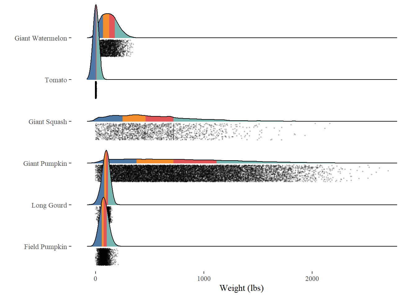

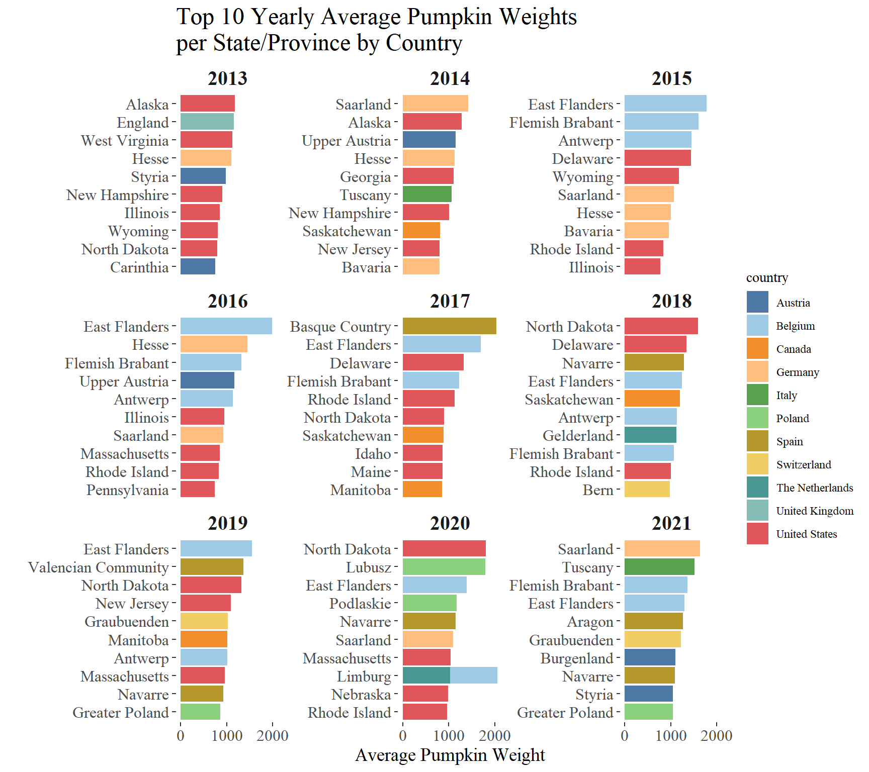
3.2 Regional and global variations in annual average weights

pumpkins |>
  group_by(year, state_prov) |>
  summarize(avg_weight = mean(weight_lbs, na.rm = T)) |>
  slice_max(avg_weight, n = 10) |>
  ungroup() |>
  inner_join(
    pumpkins |>
      select(state_prov, country),
    by = "state_prov",
    relationship = "many-to-many"
  ) |>
  distinct() |>
  mutate(state_prov = reorder_within(state_prov, avg_weight, year)) |>
  ggplot(aes(avg_weight, state_prov, fill = country)) +
  geom_col() +
  facet_wrap(. ~ year, scales = "free_y") +
  scale_y_reordered() +
  scale_fill_tableau(palette = "Tableau 20") +
  scale_x_continuous(breaks = scales::breaks_pretty(n = 3)) +
  theme(
    strip.text = element_text(size = 15, face = "bold"),
    axis.title = element_text(size = 14),
    axis.text = element_text(size = 12),
    plot.title = element_text(size = 18)
  ) +
  labs(
    x = "Average Pumpkin Weight",
    y = "",
    title = str_wrap(
      "Top 10 Yearly Average Pumpkin Weights per State/Province by Country",
      width = 40
    )
  )

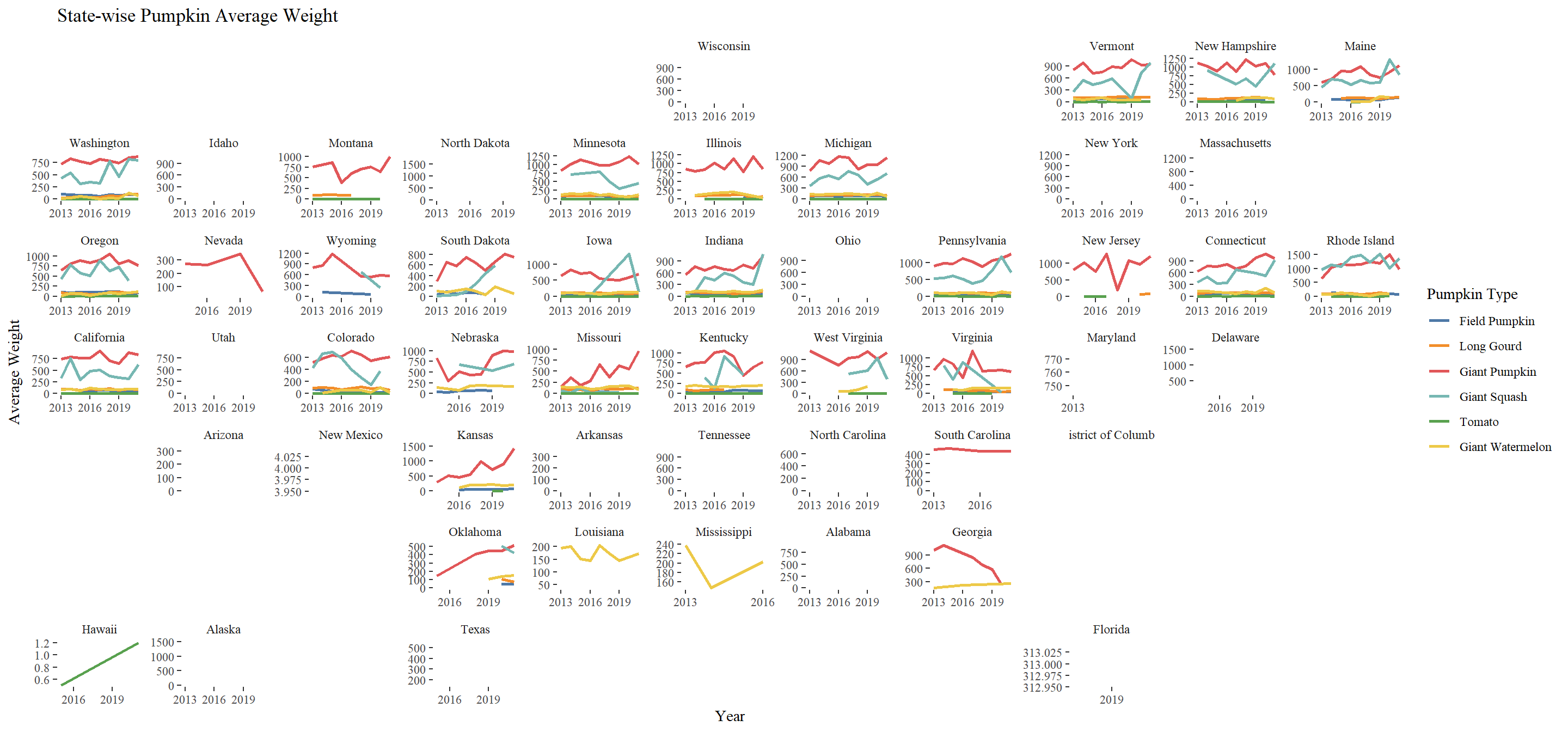
3.3 US Average Weights by State

There was a time when I really liked the idea of laying out small plots in rough map shapes. This one works out alright, but that certainly isn’t always true.

pumpkins |>
  filter(country == "United States") |>
  group_by(year, type, state_prov) |>
  summarize(avg_weight = mean(weight_lbs, na.rm = T)) |>
  ungroup() |>
  ggplot(aes(as.numeric(year), avg_weight, color = type)) +
  geom_line(linewidth = 1) +
  facet_geo(~state_prov, label = "name", scales = "free") +
  scale_x_continuous(breaks = seq(2013, 2021, 3)) +
  scale_color_tableau() +
  labs(
    x = "Year",
    y = "Average Weight",
    color = "Pumpkin Type",
    title = "State-wise Pumpkin Average Weight"
  )